| Variable | Type | Description |
|---|---|---|
| Age | Numeric | Age of the patient in years |
| Gender | Categorical | Patient gender: Male or Female |
| Polyuria | Categorical | Excessive urination: Yes or No |
| Polydipsia | Categorical | Excessive thirst: Yes or No |
| sudden weight loss | Categorical | Unexplained weight loss: Yes or No |
| weakness | Categorical | General body weakness: Yes or No |
| Polyphagia | Categorical | Excessive hunger: Yes or No |
| Genital thrush | Categorical | Fungal infection in genital area: Yes or No |
| visual blurring | Categorical | Blurred vision: Yes or No |
| Itching | Categorical | Persistent skin itching: Yes or No |
| Irritability | Categorical | Increased irritability: Yes or No |
| delayed healing | Categorical | Slow wound healing: Yes or No |
| partial paresis | Categorical | Partial muscle weakness: Yes or No |
| muscle stiffness | Categorical | Stiffness in muscles: Yes or No |
| Alopecia | Categorical | Hair loss: Yes or No |
| Obesity | Categorical | Obese body condition: Yes or No |
| class | Categorical | Diagnosis outcome: Positive or Negative for early-stage diabetes |
Abstract
Early identification of diabetes risk enables timely lifestyle and clinical interventions. Using a dataset of 520 patients with demographic and symptom indicators (e.g., polyuria, polydipsia, weakness), we develop an interpretable logistic regression model to predict early-stage diabetes. After exploratory analysis of age, gender, and symptom prevalence, we compare candidate models and finalize a specification that includes a clinically motivated interaction between polyuria and weakness. Model performance is evaluated with hold-out metrics and ROC/AUC, alongside calibration to assess reliability of predicted risks. We present adjusted odds ratios with confidence intervals to quantify each predictor’s contribution and visualize marginal effects for age and key symptoms. Results highlight strong associations for polyuria and polydipsia, a notable negative effect for male gender, and an attenuated combined effect for polyuria × weakness. We discuss implications for screening workflows and limitations related to sample size and self-reported symptoms. Overall, the model provides a transparent baseline that balances predictive utility with interpretability, suitable for early risk stratification and as a foundation for future, larger-scale studies.
Introduction
Background
Diabetes mellitus is a chronic metabolic disorder characterized by elevated blood glucose levels, which can lead to long-term damage to the heart, kidneys, eyes, and nerves. Early-stage detection is critical because timely intervention through lifestyle changes, medication, or monitoring can slow or even prevent progression to more severe stages. In clinical practice, logistic regression is one of the most widely used predictive models because of its interpretability and straightforward implementation, making it a valuable tool for risk stratification in healthcare.
Research Question
Can a logistic regression model using demographic and symptom-based predictors accurately predict the risk of early-stage diabetes in patients, and which factors contribute most strongly to that risk?
For example, given a 40-year-old female presenting with genital thrush and weakness, can the model estimate her probability of having early-stage diabetes?
Objectives
This analysis aims to:
- Explore the distribution of age, gender, and key symptoms in the study population.
- Quantify differences in symptom prevalence between patients with and without early-stage diabetes.
- Build a logistic regression model to identify significant predictors of diabetes risk.
- Evaluate model performance using classification metrics and ROC/AUC.
- Interpret results in a clinically meaningful way, including examination of an interaction between polyuria and weakness.
Data Description
Dataset Overview
The dataset contains information from 520 patients, each described by demographic information, self-reported symptoms, and a diagnosis label indicating early-stage diabetes status. The data consists of 16 predictor variables and one target variable, class, which takes the values Positive (patient has early-stage diabetes) or Negative (patient does not have early-stage diabetes).
All predictors are categorical except for Age, which is numeric and represents the patient’s age in years.
Variables
Table 1 below provides a summary of each variable, including its type and description.
Data Preparation Notes
- All categorical variables were coded as Yes or No.
- The target variable
classwas converted to a binary outcome for modeling purposes, with Positive coded as 1 and Negative as 0. - There were no missing values in the dataset.
Exploratory Data Analysis
This section summarizes key characteristics of the study population prior to modeling, focusing on demographics (age and gender) and the distribution of symptom indicators across diabetes status.
Age Distribution
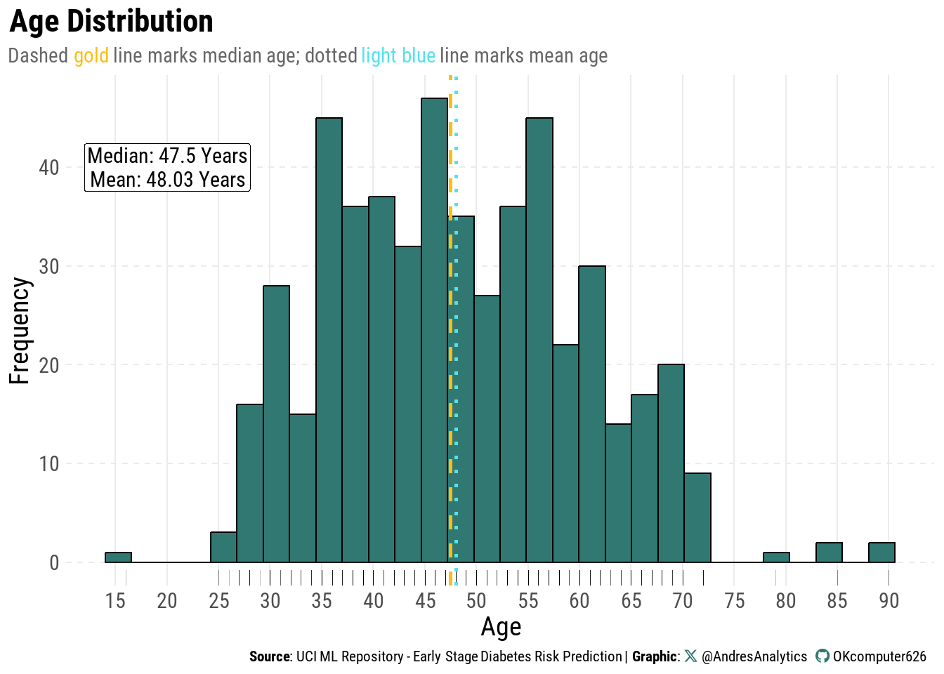
Figure 1 shows the distribution of patient ages in the study population.
Most patients are between 40 and 60 years old, with fewer younger adults and a gradual taper into the 70s–90s. The distribution is slightly right-skewed due to the presence of older individuals.
The median age is 47.5 years (gold dashed line) and the mean age is 48.03 years (light blue dotted line). Their close proximity suggests minimal skew, indicating that the age distribution is relatively balanced.
Clinically, this age profile aligns with known patterns of early-stage diabetes, which tends to be more common in middle-aged and older adults.
Age and Gender by Diabetes Status
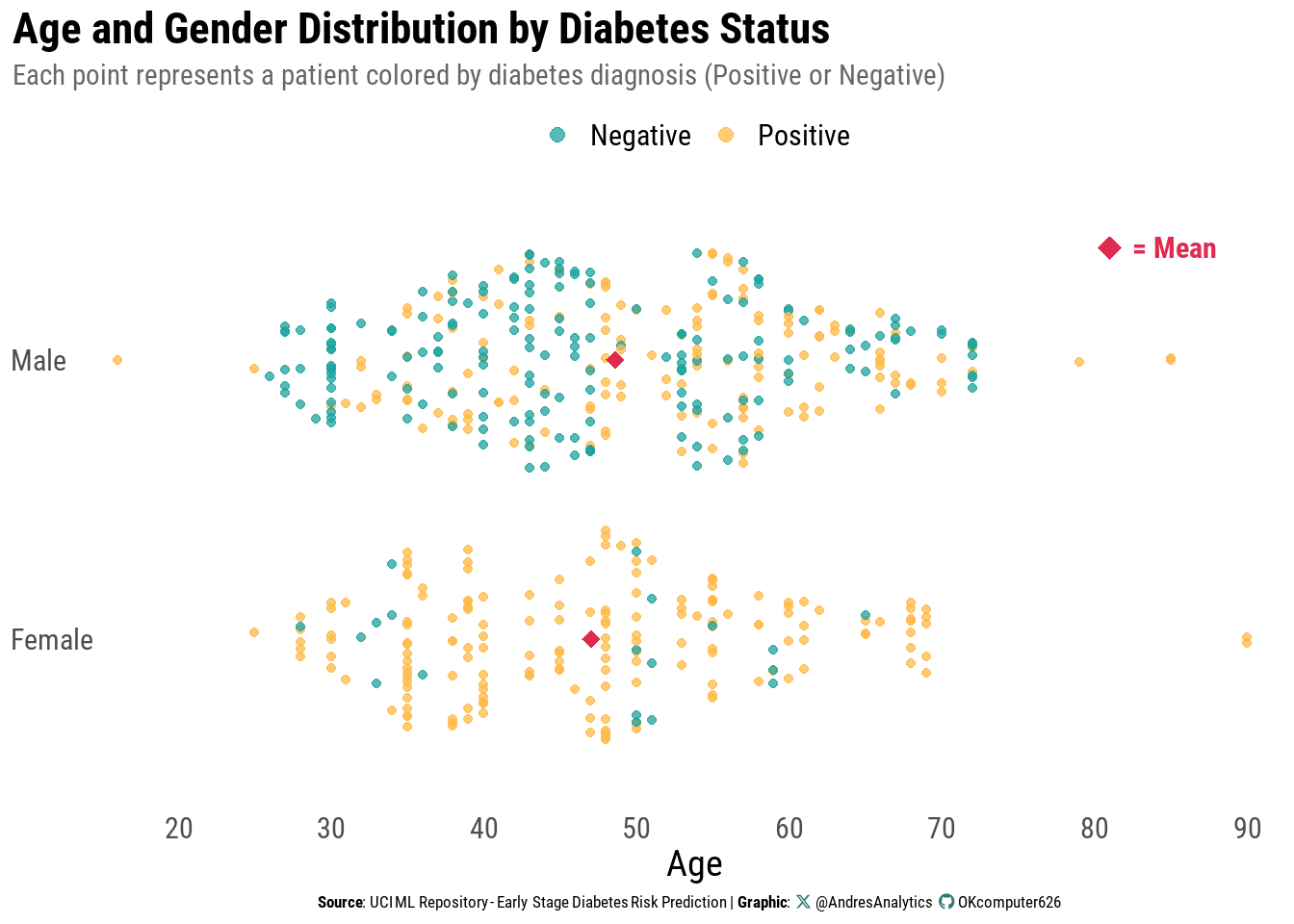
Figure 2 shows the distribution of patient ages stratified by gender, with points colored according to diabetes diagnosis (Positive or Negative).
Each dot represents an individual patient, allowing visualization of the overlap and separation of age profiles between the two outcome groups.
Key observations:
- For both males and females, positive diagnoses are more common in middle-aged and older adults, generally between 35 and 65 years.
- Negative cases are spread more evenly across ages but are less common among older adults.
- The mean age within each gender group (red diamond) is close to 47–48 years, consistent with the median and mean from the overall age distribution.
- No extreme gender imbalance in sample size is observed, but subtle shifts in age patterns by gender are visible — for example, female positive cases appear slightly younger on average than male positive cases.
From a clinical perspective, this pattern supports the established understanding that early-stage diabetes prevalence increases with age, but the relationship is nuanced when examined separately by gender.
Age Distribution by Diabetes Status
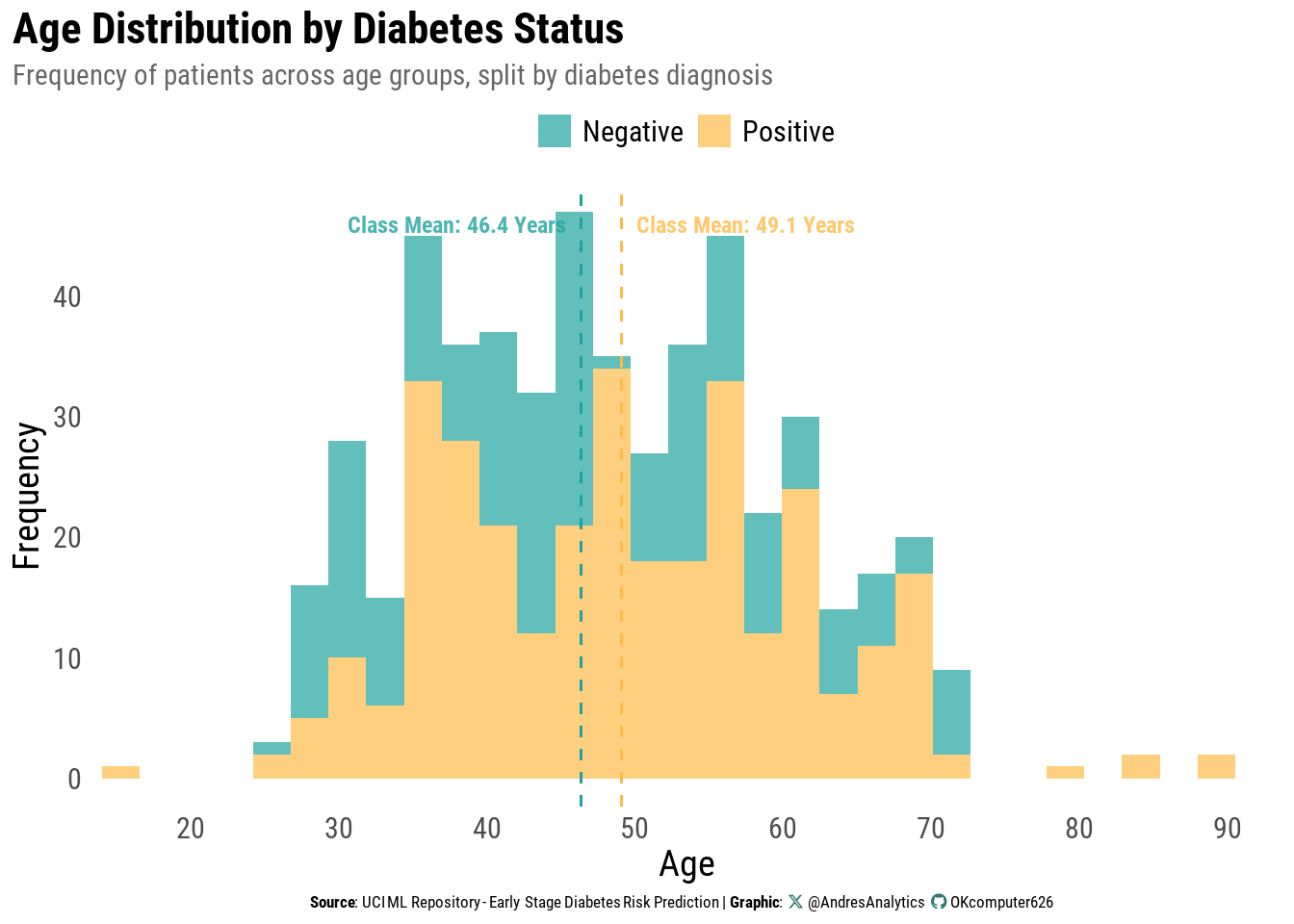
Figure 3 presents the distribution of patient ages, separated by diabetes diagnosis (Positive or Negative). The histogram shows how frequently patients occur across different age groups, with class-specific means indicated by dashed vertical lines.
Key observations:
- Patients without diabetes have a slightly lower mean age (46.4 years) than those with diabetes (49.1 years).
- Most patients in both groups are between 35 and 65 years, with fewer cases among younger adults and those over 70.
- The right tail extends into the late 80s, though cases in this range are rare.
- Overlap between groups suggests that age alone is not a strong discriminator, but the upward shift in the positive group’s mean aligns with the trend that diabetes prevalence increases with age.
From a clinical perspective, the modest age gap reflects the progressive nature of type 2 diabetes risk over the life course, even if age is not a standalone predictor.
Visual Summary of Demographics and Symptoms
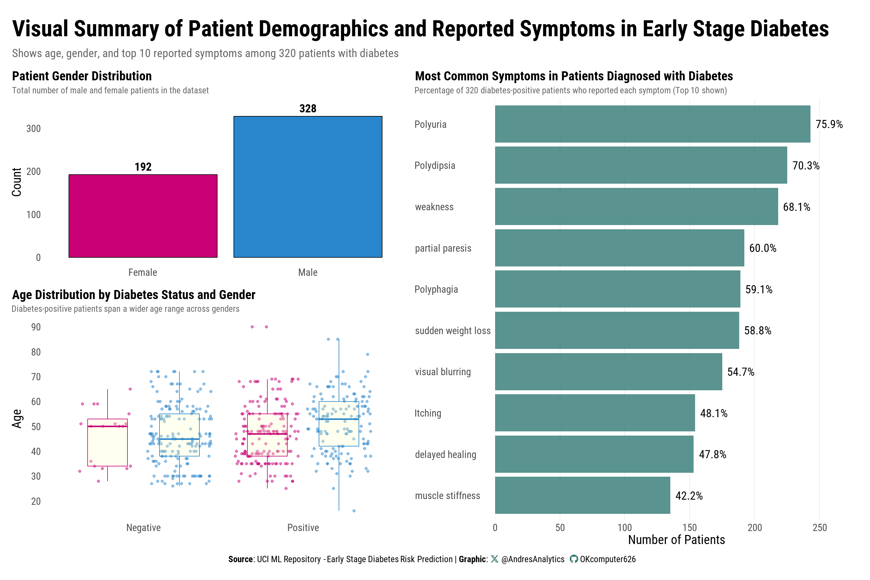
Figure 4 presents three complementary views summarizing patient demographics and symptom patterns prior to modeling.
Key observations:
- Gender composition: There is a slight predominance of male patients, which is important for interpreting model coefficients and assessing generalizability.
- Age by diabetes status and gender: Patients with diabetes span a wider age range compared to those without. While mean ages are similar across genders, positive cases—particularly among males—include a higher proportion of older adults.
- Symptom profile of positive cases: The most frequently reported symptoms are polyuria and polydipsia, followed by weakness. Other symptoms decline in prevalence and show gradual variation, suggesting that no single symptom alone is sufficient for accurate classification.
Interpretation and relevance:
- The male skew and mid-to-older age distribution align with known diabetes epidemiology, supporting the inclusion of age and gender as covariates in the logistic model.
- The symptom hierarchy matches clinical expectations, reinforcing the decision to include these indicators in the model while also motivating the exploration of clinically relevant interactions (e.g., polyuria × weakness) rather than modeling symptoms in isolation.
Next steps:
These descriptive findings guide the logistic regression specification, inform the selection of interaction terms, and set realistic expectations for effect sizes and model calibration.
Bivariate Analysis
Before specifying the logistic regression model, we examine how each predictor relates individually to diabetes status. This helps confirm expected relationships, identify unexpected patterns, and guide which variables or interactions may improve the model.
Symptom Prevalence by Diabetes Status
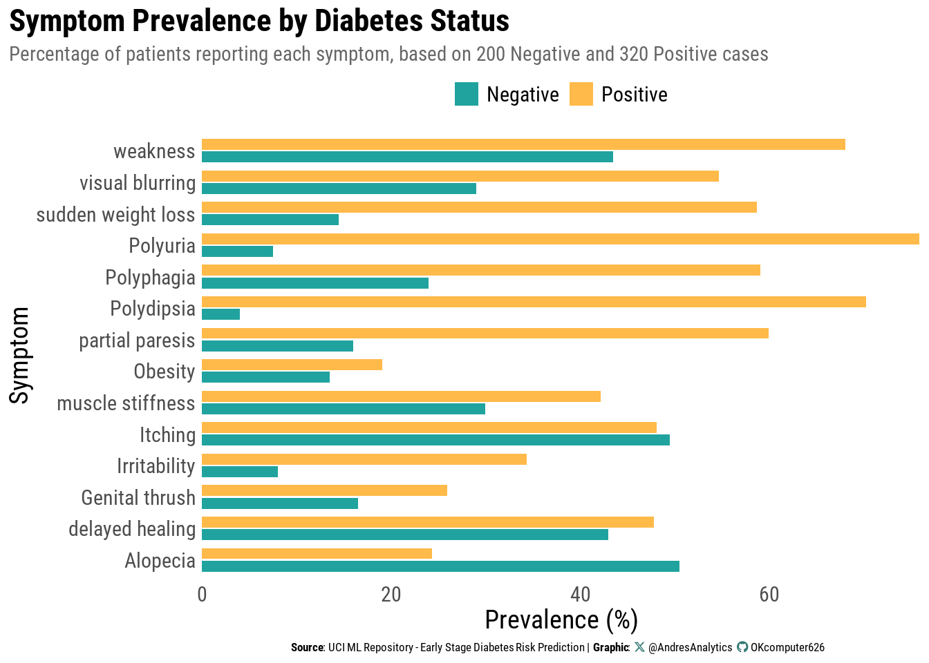
Figure 5 compares the percentage of patients reporting each symptom, separated by diagnosis group.
Key observations:
- Classic symptom dominance: Polyuria and polydipsia are far more common among diabetes-positive patients, consistent with clinical expectations.
- Broader symptom elevation: Weakness, sudden weight loss, polyphagia, and partial paresis also occur at substantially higher rates in positives than in negatives.
- Areas of overlap: Itching, delayed healing, and alopecia appear at similar rates across groups, suggesting limited standalone discriminative value.
Why it matters:
- Large prevalence gaps indicate strong candidates for inclusion in the logistic model and suggest higher odds ratios.
- Overlapping symptoms highlight the need for a multivariable approach: no single indicator is sufficient for accurate classification.
Next step:
These contrasts will help prioritize predictors and guide the inclusion of clinically motivated interactions (e.g., polyuria × weakness) in the logistic regression model.
Methods
Problem Setup and Notation
Let \(Y_i \in \{0, 1\}\) indicate early-stage diabetes status for subject \(i\),
with \(1 = \text{Positive}\) and \(0 = \text{Negative}\).
Let:
\[ x_i = (x_{i1}, \dots, x_{ip})^\top \]
denote \(p\) predictors, such as demographics, symptoms, and lifestyle factors.
We model the conditional probability of a positive diagnosis as:
\[ \Pr(Y_i = 1 \mid x_i) = p_i \]
Logistic Regression Model
Logistic regression links \(p_i\) to a linear predictor using the logit function:
\[ \text{logit}(p_i) \equiv \log\left( \frac{p_i}{1 - p_i} \right) = \eta_i = \beta_0 + \beta_1 x_{i1} + \cdots + \beta_p x_{ip} \]
Equivalently:
\[ p_i = \frac{\exp(\eta_i)}{1 + \exp(\eta_i)} \]
Here:
- \(\beta_j\) represents the change in log-odds of diabetes for a one-unit increase in \(x_{ij}\), holding all other variables constant.
- The quantity \(e^{\beta_j}\) is the odds ratio (OR), indicating the multiplicative change in odds for a one-unit change in \(x_{ij}\).
Likelihood and Estimation
Assuming independent Bernoulli outcomes given \(x_i\), the likelihood is:
\[ L(\beta) = \prod_{i=1}^{n} p_i^{y_i} (1 - p_i)^{1 - y_i} \]
and the log-likelihood is:
\[ \ell(\beta) = \sum_{i=1}^{n} \left[ y_i \log p_i + (1 - y_i) \log (1 - p_i) \right] \]
Parameters \(\beta\) are estimated by maximum likelihood, using Newton–Raphson or Iteratively Reweighted Least Squares (IRLS).
Model Building and Selection in R
All models were fitted in R using the glm() function with family = binomial.
A null model (intercept only) and a full model (all predictors) were specified.
Stepwise selection was applied in both forward and backward directions using the Akaike Information Criterion (AIC) as the selection metric:
# Refit on the full dataset using forward selection
null_model <- glm(class ~ 1, data = diabetes, family = binomial)
full_model <- glm(class ~ ., data = diabetes, family = binomial)

# Forward selection
forward_model <- stepAIC(null_model,
                       direction = "forward",
                       scope = list(lower = null_model, upper = full_model),
                       trace = FALSE)

# Backward elimination
backward_model <- stepAIC(full_model,
                       direction = "backward",
                       scope = list(lower = null_model, upper = full_model),
                       trace = FALSE)
Following selection, AIC values were compared (Table 2). The forward model achieved a slightly lower AIC (198.36) than the backward model (198.64), indicating a marginally better fit according to this criterion.
Decision: The forward-selected model was chosen for subsequent analysis.
| Model | df | AIC |
|---|---|---|
| Forward Model | 11 | 198.3606 |
| Backward Model | 13 | 198.6403 |
Final Model with Interaction
An interaction term between weakness and polyuria was added to capture whether the effect of one symptom on diabetes risk depends on the presence of the other.
Including this interaction improved model fit relative to the forward-selected main-effects model, as indicated by a lower AIC (196.24 vs. 198.36; Table 3).
Decision:
The interaction model was retained as the final model for interpretation and evaluation.
| Model | df | AIC |
|---|---|---|
| Forward Model | 11 | 198.3606 |
| Final Model | 12 | 196.2394 |
Final Logistic Regression Results
Table 4 presents odds ratios (ORs) with 95% confidence intervals (CIs) and Bonferroni-adjusted p-values for the final model, which includes the polyuria × weakness interaction.
| Characteristic | OR1 | SE | 95% CI | p-value |
|---|---|---|---|---|
| polyuria | ||||
| Yes / No | 77.3*** | 47.9 | 22.9, 261 | <0.001 |
| polydipsia | ||||
| Yes / No | 206*** | 155 | 47.4, 899 | <0.001 |
| gender | ||||
| Male / Female | 0.01*** | 0.005 | 0.00, 0.03 | <0.001 |
| itching | ||||
| Yes / No | 0.07*** | 0.037 | 0.02, 0.20 | <0.001 |
| irritability | ||||
| Yes / No | 11.3*** | 6.30 | 3.78, 33.7 | <0.001 |
| genital_thrush | ||||
| Yes / No | 7.01*** | 3.58 | 2.58, 19.1 | <0.001 |
| partial_paresis | ||||
| Yes / No | 3.62** | 1.79 | 1.38, 9.54 | 0.009 |
| polyphagia | ||||
| Yes / No | 3.72** | 1.86 | 1.39, 9.92 | 0.009 |
| age | 0.94** | 0.020 | 0.90, 0.98 | 0.006 |
| weakness | ||||
| Yes / No | 1.45 | 0.705 | 0.56, 3.76 | 0.449 |
| polyuria * weakness | ||||
| Yes * Yes | 0.14* | 0.140 | 0.02, 0.94 | 0.046 |
| Abbreviations: CI = Confidence Interval, OR = Odds Ratio, SE = Standard Error | ||||
| 1 *p<0.05; **p<0.01; ***p<0.001 | ||||
Note
How to read this: Odds ratios (OR) > 1 indicate higher odds of early-stage diabetes for the “Yes” (or first-listed) category; OR < 1 indicate lower odds, holding other variables constant. P-values are Bonferroni-adjusted.
Strongest positive associations
-
Polydipsia (excessive thirst) — OR 206 (95% CI: 47.4, 899; p < 0.001).
Individuals reporting polydipsia are over 200× more likely to have early-stage diabetes. This is the strongest predictor. -
Polyuria (frequent urination) — OR 77.3 (22.9, 261; p < 0.001).
Very large increase in odds, consistent with classic symptomatology. - Irritability — OR 11.3 (3.78, 33.7; p < 0.001).
- Genital thrush — OR 7.01 (2.58, 19.1; p < 0.001).
- Polyphagia (excessive hunger) — OR 3.72 (1.39, 9.92; p = 0.009).
- Partial paresis — OR 3.62 (1.38, 9.54; p = 0.009).
Negative associations
-
Male vs Female — OR 0.01 (0.00, 0.03; p < 0.001).
Males show markedly lower odds than females in this dataset. -
Itching — OR 0.07 (0.02, 0.20; p < 0.001).
Associated with substantially reduced odds. -
Age (per year) — OR 0.94 (0.90, 0.98; p = 0.006).
Slight decrease (~6% per year). Note: Counterintuitive; likely reflects sample characteristics rather than a generalizable trend.
Interaction
-
Polyuria × Weakness — OR 0.14 (0.02, 0.94; p = 0.046).
The combined presence of polyuria and weakness yields lower odds than expected from adding their individual effects. Practically, weakness attenuates the otherwise strong association between polyuria and diabetes.
Non-significant
-
Weakness (main effect) — OR 1.45 (0.56, 3.76; p = 0.449).
Not significant after adjustment when considered on its own.
Tip
Bottom line: Classic symptoms—polydipsia and polyuria—dominate risk prediction by large margins. Additional symptoms (irritability, genital thrush, polyphagia, partial paresis) contribute meaningfully. Sex, itching, and age show protective associations in this sample, and the polyuria × weakness interaction suggests that weakness moderates polyuria’s effect.
Visual Interpretation
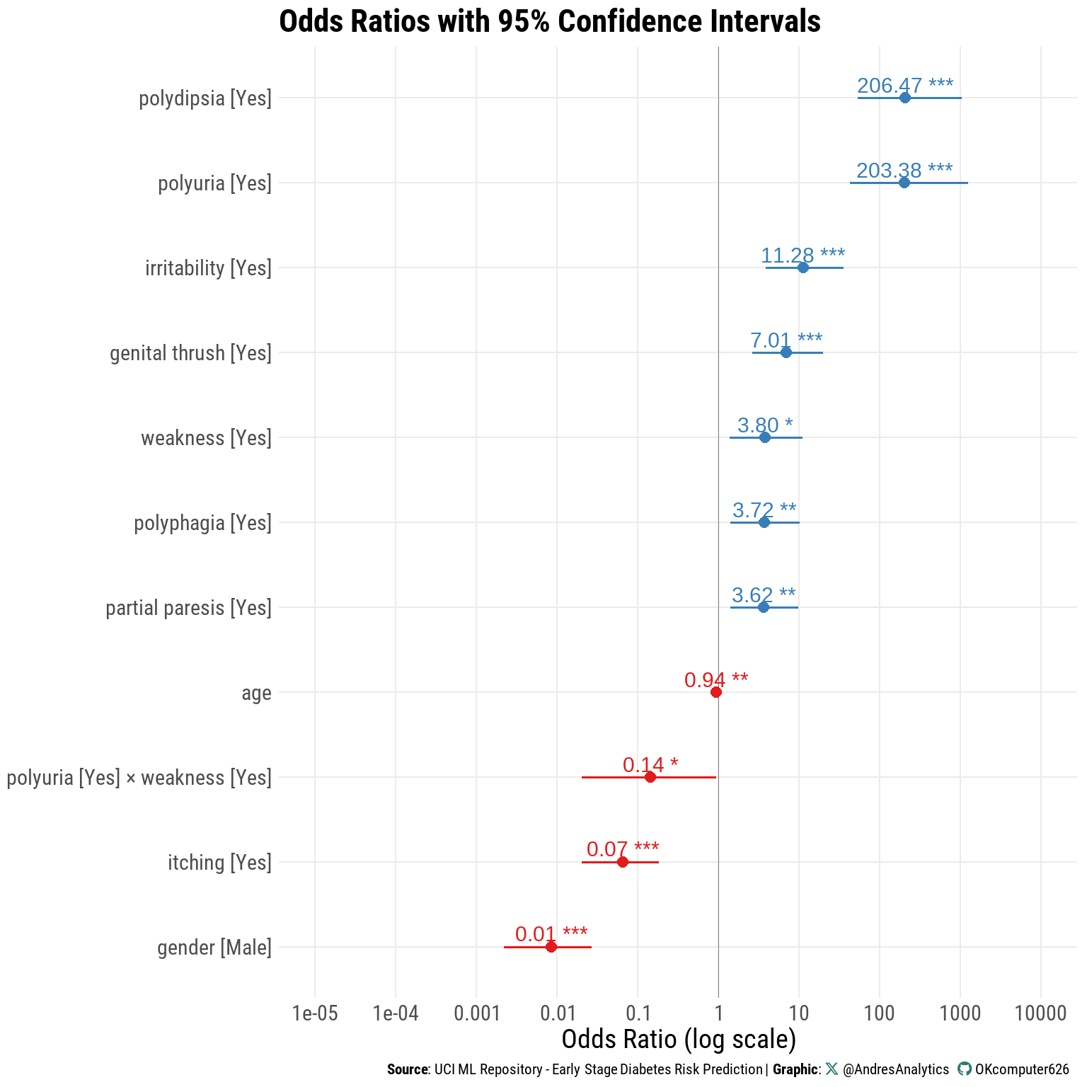
Figure 6 visually summarizes the final logistic regression model’s odds ratios (log scale) with 95% confidence intervals.
- Polydipsia and Polyuria are positioned far to the right, confirming their exceptionally strong positive associations with early-stage diabetes.
- Other predictors with elevated odds include Irritability, Genital Thrush, Weakness, Polyphagia, and Partial Paresis.
- Negative associations — Male gender, Itching, Age, and the Polyuria × Weakness interaction — appear to the left of the 1.0 reference line, indicating reduced odds.
- The log scale emphasizes the large gap between the strongest predictors and those with more moderate effects.
- Confidence interval widths reflect precision: narrower intervals suggest more reliable estimates, while wider intervals (e.g., for polydipsia and polyuria) indicate greater variability in the data.
Takeaway:
The plot complements the odds ratio table by illustrating the magnitude and direction of each predictor’s effect, while also conveying the relative precision of these estimates.
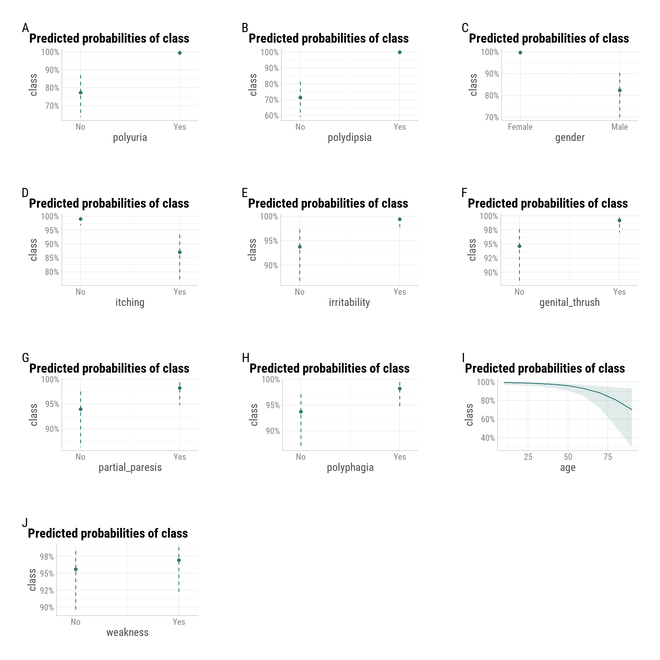
Predicted Probabilities by Predictor
Marginal effects plots display the model-implied probability of early-stage diabetes for each predictor, averaging over other variables in the model.
- Polyuria and Polydipsia have the strongest effects, with “Yes” responses pushing predicted probability close to 100%.
- Gender shows markedly lower predicted probability for males, consistent with the negative odds ratio in the regression results.
- Irritability, Genital Thrush, Partial Paresis, and Polyphagia each raise predicted probability by several percentage points.
- Itching is associated with a noticeably lower predicted probability, matching its protective effect in the model.
- Weakness has only a modest positive shift in predicted probability.
- Age shows a declining curve, with lower predicted probabilities at older ages, reinforcing the non-linear pattern identified in the GAM analysis.
Takeaway:
The marginal effects confirm that polyuria and polydipsia dominate risk prediction, while other symptoms and demographic factors contribute smaller but consistent influences on predicted diabetes probability.
Model Evaluation
Model Diagnostics
Exploring Non-Linear Effects (GAM Analysis)
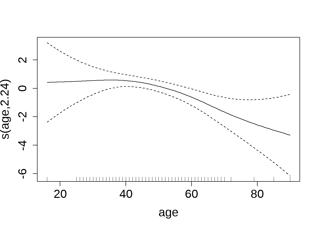
To assess whether the relationship between age and early-stage diabetes risk is strictly linear, we fit a Generalized Additive Model (GAM) including a smooth term for age, as shown in Figure 8.
The smooth function indicates:
- Ages ~20–40: Log-odds remain relatively flat, suggesting minimal effect.
- After ~40: A gradual downward slope emerges, indicating a decrease in diabetes risk with increasing age—consistent with the negative linear estimate from the logistic regression.
- Extremes (<25 or >80 years): Wider confidence intervals reflect greater uncertainty due to fewer observations.
Takeaway:
While the logistic regression treated age as a strictly linear predictor, the GAM reveals that the decline in risk is more pronounced in older adults, with little effect in younger to mid-age ranges.
Overall Model Fit and Assumption Checks
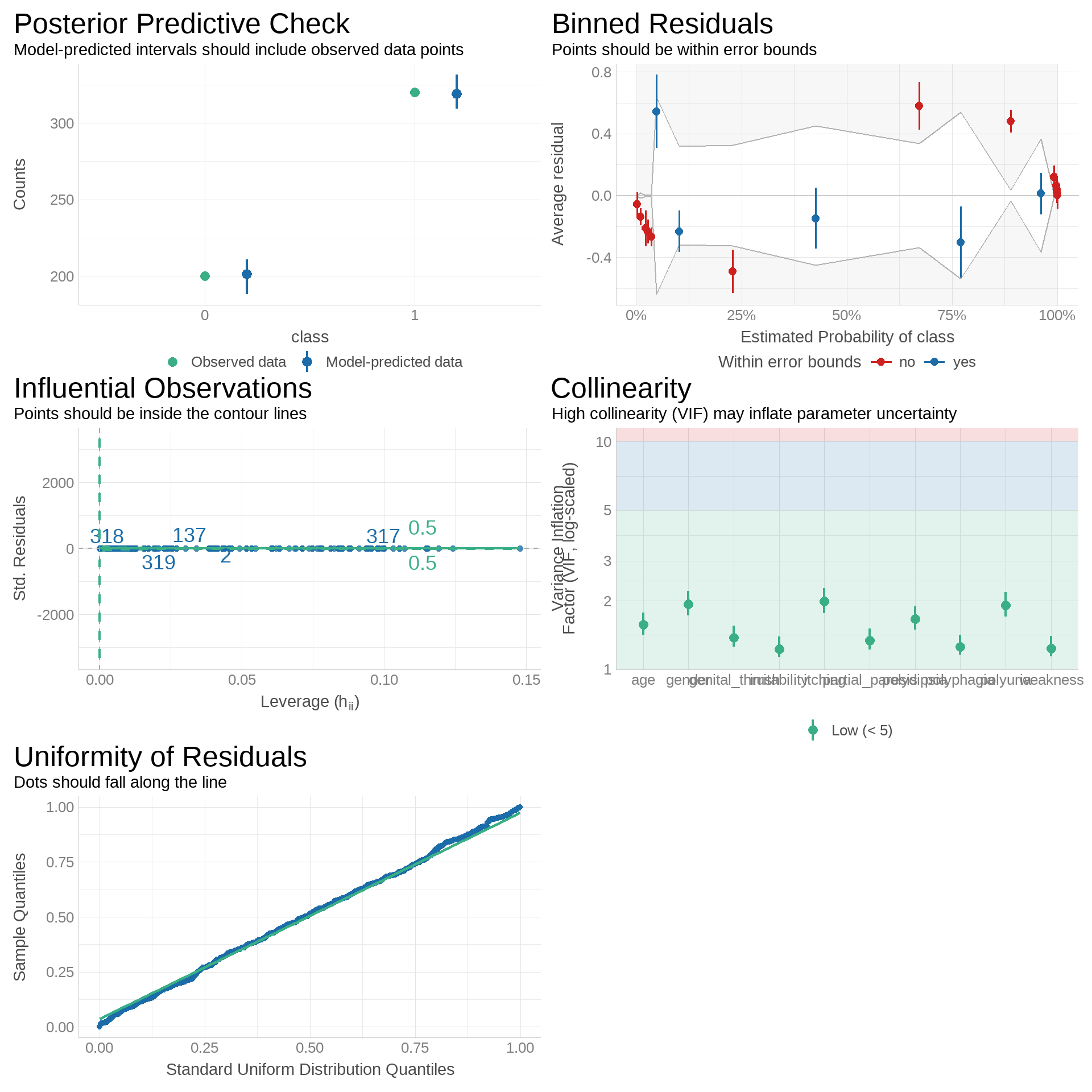
We evaluated model fit, assumptions, and stability using several diagnostic checks, as shown in Figure 9:
-
Posterior Predictive Check:
Predicted intervals cover the observed class counts, indicating good calibration between model predictions and actual outcomes. -
Binned Residuals:
Most residual averages fall within error bounds, with minor deviations at probability extremes. This suggests the model is generally well-calibrated but may underfit certain ranges. -
Influential Observations:
All points lie within contour lines on the leverage vs. standardized residuals plot, indicating no single observation exerts undue influence. -
Collinearity (VIF):
All Variance Inflation Factor values are below 5, suggesting low multicollinearity and stable coefficient estimation. -
Uniformity of Residuals (Q–Q Plot):
Residual quantiles closely follow the standard uniform distribution, supporting the assumption of well-behaved residuals.
Summary:
Diagnostics confirm that the model is well-specified, stable, and free from serious violations, with only minor residual patterning at probability extremes that may merit further investigation.
Model Performance
The model achieved high overall performance, correctly classifying 94.8% of cases with strong sensitivity (93.0%) and specificity (95.9%) as shown in Table 5.
| Metric | Value | Description |
|---|---|---|
| Accuracy | 0.948 | How often the model predicts correctly |
| Sensitivity (Recall) | 0.930 | How well it identifies positive cases |
| Specificity | 0.959 | How well it identifies negative cases |
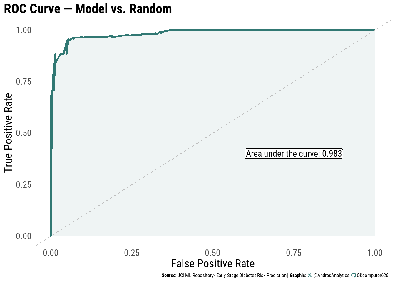
ROC Curve
The Receiver Operating Characteristic (ROC) curve (Figure 10) evaluates the model’s ability to discriminate between positive and negative cases.
The model achieved an area under the curve (AUC) of:
\[ \text{AUC} = 0.983 \]
This indicates excellent discrimination and near-perfect classification performance.
Train–Test Evaluation
Using an 80/20 split, the model achieved a train accuracy of \(0.945\), test accuracy of \(0.962\), and a test AUC of \(0.982\).
The close alignment between training and test performance, as shown in Table 6, indicates that the model is capturing genuine patterns in the data rather than memorizing noise, with little evidence of overfitting.
This balance suggests the model should maintain its predictive strength when applied to new, unseen cases.
| Model Evaluation Metrics | ||
| Metric | Value | Description |
|---|---|---|
| Train Accuracy | 0.945 | Accuracy on the training set |
| Test Accuracy | 0.962 | Accuracy on the test set |
| Test AUC | 0.982 | Area under the ROC curve for test set |
Discussion
The final logistic regression model demonstrated high predictive performance (Accuracy 94.8%, Sensitivity 93.0%, Specificity 95.9%, AUC 0.983), indicating excellent discrimination between diabetes-positive and diabetes-negative cases.
In line with established clinical knowledge, polydipsia and polyuria were the strongest predictors of early-stage diabetes risk, followed by irritability, genital thrush, polyphagia, and partial paresis. Protective associations were observed for male gender, itching, and increasing age. The polyuria × weakness interaction suggested that when both symptoms occur together, the increase in odds is smaller than expected from their individual effects.
Scenario comparison: For two otherwise identical 40-year-old patients with genital thrush and weakness (all other symptoms absent), the model predicts a higher probability for the female than for the male (Table 7, Figure 11). This aligns with the strong protective association for male gender in the final model. Genital thrush alone is associated with markedly higher odds of early-stage diabetes (OR = 7.01), and while weakness has a more modest effect, the combination still elevates risk compared to patients without these symptoms. The absence of polyuria and polydipsia in this scenario results in a lower overall predicted probability than cases where those hallmark symptoms are present.
Worked Example: Scenario Prediction by Gender
We compare two identical profiles—age 40, genital thrush = Yes, weakness = Yes, all other symptoms = No—that differ only by gender.
Given the strong protective effect for males in the final model, the male is expected to have a lower predicted probability than the female, all else equal.
| Scenario Prediction by Gender (Logistic Regression) | |||||||||||
| Scenario | gender | age | genital_thrush | weakness | polyuria | polydipsia | itching | irritability | partial_paresis | polyphagia | Predicted_Probability |
|---|---|---|---|---|---|---|---|---|---|---|---|
| 40F: GT Yes, Weakness Yes; others No | Female | 40 | Yes | Yes | No | No | No | No | No | No | 0.981 |
| 40M: GT Yes, Weakness Yes; others No | Male | 40 | Yes | Yes | No | No | No | No | No | No | 0.309 |
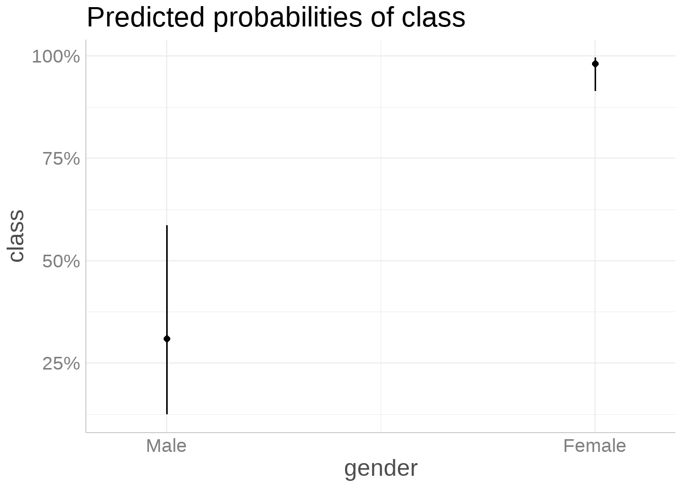
Scenario takeaway: Holding all other symptoms constant (genital thrush and weakness present; others absent) at age 40, the model predicts a lower probability for the male than the female (Table 7, Figure 11), consistent with the protective association for males observed in the final model.
Limitations
While the final logistic regression model demonstrated strong predictive performance and clinical interpretability, several limitations should be considered when interpreting the results:
-
Sample size and diversity: The dataset contains \(n = 520\) observations, which is adequate for model training but still limits representation of certain demographic groups and rare symptom combinations. This may affect the model’s generalizability to broader populations.
-
Self-reported symptoms: Predictors such as polyuria, polydipsia, and irritability rely on self-reported data, which can introduce recall bias or misclassification.
-
Cross-sectional design: The analysis is based on a single time-point per patient, preventing assessment of symptom changes or progression of diabetes risk over time.
-
Missing socioeconomic and demographic factors: Variables such as family income, race/ethnicity, and location of residence were not available. These factors are known to influence health outcomes and could improve predictive accuracy and fairness if included.
-
Model scope: Only demographic and symptom-based predictors were included; laboratory results (e.g., fasting glucose, HbA1c) and lifestyle factors were excluded, which could enhance model performance.
- External validation: The model has not yet been validated on an independent dataset. As such, reported performance metrics may be optimistic when applied to new, unseen populations.
Summary:
These limitations suggest that while the model is promising for early screening, further work is needed to validate it in larger and more diverse populations, incorporate socioeconomic and geographic factors, and confirm its robustness outside the development dataset.
Conclusion
This study set out to answer two primary research questions:
- Can a logistic regression model using demographic and symptom-based predictors accurately predict the risk of early-stage diabetes in patients?
- How would the model estimate diabetes risk for specific patient scenarios, such as two otherwise identical individuals differing only by gender?
The final model achieved high predictive performance—Accuracy = 94.8%, Sensitivity = 93.0%, Specificity = 95.9%, and AUC = 0.983—indicating excellent discrimination between diabetes-positive and diabetes-negative cases. Consistent with established clinical knowledge, polydipsia and polyuria emerged as the most influential predictors, followed by irritability, genital thrush, polyphagia, and partial paresis. Male gender, itching, and increasing age showed protective associations.
Scenario-based predictions reinforced the model’s interpretability. When comparing two identical patients—both aged 40, with genital thrush and weakness, and all other symptoms absent—the model predicted a higher probability of early-stage diabetes for the female than for the male, consistent with the protective effect associated with male gender.
These findings suggest that symptom-based logistic regression models can serve as effective decision-support tools for identifying patients at elevated risk, particularly when hallmark symptoms such as polyuria and polydipsia are present. However, as discussed in the Limitations section, additional demographic and socioeconomic factors, as well as broader data diversity, could further enhance model generalizability and clinical utility.
Overall, the results demonstrate that relatively simple, interpretable models can yield strong predictive accuracy, offering both actionable insights for clinicians and a foundation for future predictive modeling work in diabetes risk assessment.
References
Dua, D., & Graff, C. (2019). UCI Machine Learning Repository: Early Stage Diabetes Risk Prediction Dataset. University of California, Irvine. Retrieved from https://archive.ics.uci.edu/
Pagano, M., & Gauvreau, K. (2000). Principles of Biostatistics (2nd ed.). Harvard School of Public Health & Harvard Medical School.
Wickham, H., Averick, M., Bryan, J., Chang, W., McGowan, L., François, R., Grolemund, G., Hayes, A., Henry, L., Hester, J., Kuhn, M., Pedersen, T. L., Miller, E., Bache, S. M., Müller, K., Ooms, J., Robinson, D., Seidel, D. P., Spinu, V., … Yutani, H. (2019). Welcome to the tidyverse. Journal of Open Source Software, 4(43), 1686. https://doi.org/10.21105/joss.01686
Riswanto, U. (2025, April 20). A Beginner’s Guide to Multivariate Logistic Regression in R. Medium. Retrieved from https://ujangriswanto08.medium.com/a-beginners-guide-to-multivariate-logistic-regression-in-r-9aa3b763f564
yuzaR Data Science. (2024, October 2). Multivariable Logistic Regression in R: The Ultimate Masterclass (4K)! [YouTube video]. Retrieved from https://www.youtube.com/watch?v=EIR9zN0tDPw&t=420s
Citation
For attribution, please cite this work as:
Gonzalez, Andres. 2025. “Predicting Early Stage Diabetes Risk
Using Logistic Regression.” August 8, 2025. https://andresgonzalezstats.com/project/Projects/2025/Logistic
Regression/Predicting Early Stage Diabetes Risk Using Logistic
Regression.html.